8.2. An end-to-end time series analysis
In this example, we’re going to look at why the pmdarima.arima.auto_arima() method
should not be used as a silver bullet, and why qualitative investigation of the data
may reveal important characteristics about it which may, in turn, affect how you approach
the problem.
For this problem, we’ll use the pmdarima.datasets.load_sunspots() method, which
loads a seasonal time series of monthly mean relative sunspot numbers from 1749 to 1983.
Here’s what you’ll need to run this example:
- Pmdarima 1.5.2+ (many plotting utilities were added in this version)
- Matplotlib - It’s not a hard requirement of the package itself, but you’ll need it to run these examples (if you’re running this in a notebook, make sure to include
%matplotlib inline)- Python 3.6+. If you’re running python 3.5, simply remove the F-string print statements and it will work.
8.2.1. Imports, data loading & splitting
Here’s the set up for our problem. We’ll load the data and split it into our train/test sets:
import numpy as np
import pandas as pd
import matplotlib.pyplot as plt
# %matplotlib inline

import pmdarima as pm
from pmdarima.datasets import load_sunspots
from pmdarima.model_selection import train_test_split
print(f"Using pmdarima {pm.__version__}")
# Using pmdarima 1.5.2

y = load_sunspots(True)
train_len = 2750
y_train, y_test = train_test_split(y, train_size=train_len)
y_train.head()
| Jan 1749 | 58.0 |
| Feb 1749 | 62.6 |
| Mar 1749 | 70.0 |
| Apr 1749 | 55.7 |
| May 1749 | 85.0 |
| dtype: | float64 |
Time series data is a bit different from traditional machine learning in the sense that it’s temporally sensitive. That means the larger our test set, the higher we would expect our error to be for later forecasts, since our model won’t be able to effectively forecast for too many periods into the future.
For this example, we’ll take the first 2750 samples for training, and leave the last 70 as our test set.
8.2.2. Examining the data
Pmdarima 1.5.2 introduced a handy utility for visualizing your time series data:
pmdarima.utils.vizualization.tsdisplay(). We can use this to visalize our data,
take a look at the auto-correlation plot, and see the histogram of values:
from pmdarima.utils import tsdisplay

tsdisplay(y_train, lag_max=100)
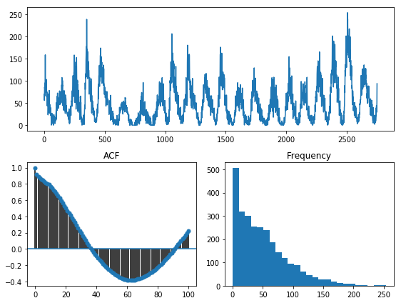
Reading this plot can give us several pieces of information:
- We are looking at a seasonal time series. Our apriori knowledge of the dataset informs
us that this data has a seasonal periodicity of
m=12. - There seems to be some significant data skew, looking at the histogram. It is very zero-inflated. A lot of the statistical techniques used in time series modeling behave better when the data is normally distributed, so this may be something to look into.
8.2.3. Fitting a baseline
Before we start manipulating our data, let’s examine what would happen if we just fit a model straight out of the box:
fit1 = pm.auto_arima(y_train, m=12, trace=True, suppress_warnings=True)
Fit ARIMA: order=(2, 1, 2) seasonal_order=(1, 0, 1, 12); AIC=22834.181, BIC=22881.533, Fit time=7.496 seconds
Fit ARIMA: order=(0, 1, 0) seasonal_order=(0, 0, 0, 12); AIC=23347.880, BIC=23359.718, Fit time=0.053 seconds
Fit ARIMA: order=(1, 1, 0) seasonal_order=(1, 0, 0, 12); AIC=23087.391, BIC=23111.067, Fit time=0.458 seconds
Fit ARIMA: order=(0, 1, 1) seasonal_order=(0, 0, 1, 12); AIC=22931.725, BIC=22955.401, Fit time=1.314 seconds
Fit ARIMA: order=(0, 1, 0) seasonal_order=(0, 0, 0, 12); AIC=23345.881, BIC=23351.800, Fit time=0.030 seconds
Fit ARIMA: order=(2, 1, 2) seasonal_order=(0, 0, 1, 12); AIC=22834.415, BIC=22875.848, Fit time=6.067 seconds
Fit ARIMA: order=(2, 1, 2) seasonal_order=(1, 0, 0, 12); AIC=22834.465, BIC=22875.898, Fit time=8.268 seconds
Fit ARIMA: order=(2, 1, 2) seasonal_order=(2, 0, 1, 12); AIC=22842.107, BIC=22895.378, Fit time=34.407 seconds
Near non-invertible roots for order (2, 1, 2)(2, 0, 1, 12); setting score to inf (at least one inverse root too close to the border of the unit circle: 0.995)
Fit ARIMA: order=(2, 1, 2) seasonal_order=(1, 0, 2, 12); AIC=22844.771, BIC=22898.042, Fit time=28.426 seconds
Near non-invertible roots for order (2, 1, 2)(1, 0, 2, 12); setting score to inf (at least one inverse root too close to the border of the unit circle: 0.997)
Fit ARIMA: order=(2, 1, 2) seasonal_order=(0, 0, 0, 12); AIC=22832.862, BIC=22868.375, Fit time=2.334 seconds
Fit ARIMA: order=(1, 1, 2) seasonal_order=(0, 0, 0, 12); AIC=22896.004, BIC=22925.599, Fit time=0.658 seconds
Fit ARIMA: order=(2, 1, 1) seasonal_order=(0, 0, 0, 12); AIC=22895.198, BIC=22924.793, Fit time=0.567 seconds
Fit ARIMA: order=(3, 1, 2) seasonal_order=(0, 0, 0, 12); AIC=22830.683, BIC=22872.115, Fit time=2.810 seconds
Fit ARIMA: order=(3, 1, 2) seasonal_order=(1, 0, 0, 12); AIC=22832.671, BIC=22880.023, Fit time=8.964 seconds
Fit ARIMA: order=(3, 1, 2) seasonal_order=(0, 0, 1, 12); AIC=22832.590, BIC=22879.942, Fit time=8.747 seconds
Fit ARIMA: order=(3, 1, 2) seasonal_order=(1, 0, 1, 12); AIC=22834.543, BIC=22887.814, Fit time=8.893 seconds
Near non-invertible roots for order (3, 1, 2)(1, 0, 1, 12); setting score to inf (at least one inverse root too close to the border of the unit circle: 0.998)
Fit ARIMA: order=(3, 1, 1) seasonal_order=(0, 0, 0, 12); AIC=22895.344, BIC=22930.857, Fit time=0.997 seconds
Fit ARIMA: order=(4, 1, 2) seasonal_order=(0, 0, 0, 12); AIC=22829.697, BIC=22877.049, Fit time=3.447 seconds
Fit ARIMA: order=(4, 1, 2) seasonal_order=(1, 0, 0, 12); AIC=22831.750, BIC=22885.021, Fit time=11.401 seconds
Fit ARIMA: order=(4, 1, 2) seasonal_order=(0, 0, 1, 12); AIC=22831.704, BIC=22884.975, Fit time=9.325 seconds
Fit ARIMA: order=(4, 1, 2) seasonal_order=(1, 0, 1, 12); AIC=22832.081, BIC=22891.271, Fit time=13.537 seconds
Near non-invertible roots for order (4, 1, 2)(1, 0, 1, 12); setting score to inf (at least one inverse root too close to the border of the unit circle: 0.999)
Fit ARIMA: order=(4, 1, 1) seasonal_order=(0, 0, 0, 12); AIC=22897.185, BIC=22938.618, Fit time=1.096 seconds
Fit ARIMA: order=(5, 1, 2) seasonal_order=(0, 0, 0, 12); AIC=22899.855, BIC=22953.126, Fit time=2.716 seconds
Fit ARIMA: order=(4, 1, 3) seasonal_order=(0, 0, 0, 12); AIC=22834.222, BIC=22887.493, Fit time=4.503 seconds
Fit ARIMA: order=(3, 1, 3) seasonal_order=(0, 0, 0, 12); AIC=22890.085, BIC=22937.437, Fit time=3.098 seconds
Fit ARIMA: order=(5, 1, 1) seasonal_order=(0, 0, 0, 12); AIC=22898.389, BIC=22945.741, Fit time=1.600 seconds
Fit ARIMA: order=(5, 1, 3) seasonal_order=(0, 0, 0, 12); AIC=22894.744, BIC=22953.934, Fit time=4.333 seconds
Examining the summary gives us:
fit1.summary()
                           Statespace Model Results
==============================================================================
Dep. Variable:                      y   No. Observations:                 2750
Model:               SARIMAX(4, 1, 2)   Log Likelihood              -11406.849
Date:                Fri, 13 Dec 2019   AIC                          22829.697
Time:                        07:46:18   BIC                          22877.049
Sample:                             0   HQIC                         22846.806
                               - 2750
Covariance Type:                  opg
==============================================================================
                 coef    std err          z      P>|z|      [0.025      0.975]
------------------------------------------------------------------------------
intercept      0.0012      0.012      0.104      0.917      -0.022       0.024
ar.L1          1.3845      0.025     55.356      0.000       1.335       1.433
ar.L2         -0.3867      0.027    -14.352      0.000      -0.440      -0.334
ar.L3         -0.0085      0.025     -0.340      0.734      -0.058       0.040
ar.L4         -0.0394      0.017     -2.264      0.024      -0.073      -0.005
ma.L1         -1.8193      0.020    -91.747      0.000      -1.858      -1.780
ma.L2          0.8570      0.020     42.443      0.000       0.817       0.897
sigma2       235.3266      4.006     58.739      0.000     227.474     243.179
===================================================================================
Ljung-Box (Q):                       79.17   Jarque-Bera (JB):              1261.11
Prob(Q):                              0.00   Prob(JB):                         0.00
Heteroskedasticity (H):               1.21   Skew:                             0.31
Prob(H) (two-sided):                  0.00   Kurtosis:                         6.26
===================================================================================

Warnings:
[1] Covariance matrix calculated using the outer product of gradients (complex-step).
8.2.4. Transforming our data
Since we expect our model to perform better over more normal data, let’s experiment with log transformations and the Box-Cox transformation, each of which is provided as an endogenous transformer in the Pmdarima package.
from pmdarima.preprocessing import LogEndogTransformer

y_train_log, _ = LogEndogTransformer(lmbda=1e-6).fit_transform(y_train)
tsdisplay(y_train_log, lag_max=100)
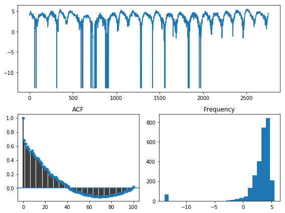
Hmm… The log transformation didn’t seem to help too much. In fact, it seems like it just
shifted the skew to the other tail. Let’s try the Box-Cox transformation. When .fit() is called,
it will learn the lambda transformation parameter:
from pmdarima.preprocessing import BoxCoxEndogTransformer

y_train_bc, _ = BoxCoxEndogTransformer(lmbda2=1e-6).fit_transform(y_train)
tsdisplay(y_train_bc, lag_max=100)
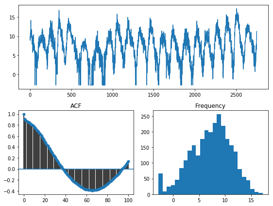
However, the Box-Cox transformation seems to work very well as a means to normalize the data! In fact, a test of normality shows overwhelmingly that this is a normal distribution:
from scipy.stats import normaltest
normaltest(y_train_bc)[1]
# 3.751017646057429e-14
8.2.5. Fitting the transformed data
Pmdarima implements a scikit-learn-esque pipeline used to chain transformations and estimators together. Using this, we can centralize the entire transformer/model fit into one metaestimator:
from pmdarima.pipeline import Pipeline

fit2 = Pipeline([
    ('boxcox', BoxCoxEndogTransformer(lmbda2=1e-6)),
    ('arima', pm.AutoARIMA(trace=True,
                           suppress_warnings=True,
                           m=12))
])

fit2.fit(y_train)
Fit ARIMA: order=(2, 1, 2) seasonal_order=(1, 0, 1, 12); AIC=9944.949, BIC=9992.301, Fit time=9.227 seconds
Fit ARIMA: order=(0, 1, 0) seasonal_order=(0, 0, 0, 12); AIC=10560.255, BIC=10572.093, Fit time=0.049 seconds
Fit ARIMA: order=(1, 1, 0) seasonal_order=(1, 0, 0, 12); AIC=10190.842, BIC=10214.518, Fit time=0.541 seconds
Fit ARIMA: order=(0, 1, 1) seasonal_order=(0, 0, 1, 12); AIC=10000.189, BIC=10023.865, Fit time=1.834 seconds
Fit ARIMA: order=(0, 1, 0) seasonal_order=(0, 0, 0, 12); AIC=10558.255, BIC=10564.174, Fit time=0.057 seconds
Fit ARIMA: order=(2, 1, 2) seasonal_order=(0, 0, 1, 12); AIC=9944.067, BIC=9985.500, Fit time=7.050 seconds
Fit ARIMA: order=(2, 1, 2) seasonal_order=(0, 0, 0, 12); AIC=9942.145, BIC=9977.659, Fit time=2.284 seconds
Fit ARIMA: order=(2, 1, 2) seasonal_order=(1, 0, 0, 12); AIC=9944.073, BIC=9985.506, Fit time=7.021 seconds
Fit ARIMA: order=(1, 1, 2) seasonal_order=(0, 0, 0, 12); AIC=9987.000, BIC=10016.595, Fit time=0.626 seconds
Fit ARIMA: order=(2, 1, 1) seasonal_order=(0, 0, 0, 12); AIC=9986.300, BIC=10015.895, Fit time=0.697 seconds
Fit ARIMA: order=(3, 1, 2) seasonal_order=(0, 0, 0, 12); AIC=9938.391, BIC=9979.824, Fit time=2.610 seconds
Fit ARIMA: order=(3, 1, 2) seasonal_order=(1, 0, 0, 12); AIC=9939.926, BIC=9987.278, Fit time=12.276 seconds
Fit ARIMA: order=(3, 1, 2) seasonal_order=(0, 0, 1, 12); AIC=9939.653, BIC=9987.005, Fit time=8.903 seconds
Fit ARIMA: order=(3, 1, 2) seasonal_order=(1, 0, 1, 12); AIC=9941.966, BIC=9995.237, Fit time=12.801 seconds
Near non-invertible roots for order (3, 1, 2)(1, 0, 1, 12); setting score to inf (at least one inverse root too close to the border of the unit circle: 0.996)
Fit ARIMA: order=(3, 1, 1) seasonal_order=(0, 0, 0, 12); AIC=9982.150, BIC=10017.664, Fit time=0.734 seconds
Fit ARIMA: order=(4, 1, 2) seasonal_order=(0, 0, 0, 12); AIC=9985.360, BIC=10032.711, Fit time=2.084 seconds
Fit ARIMA: order=(3, 1, 3) seasonal_order=(0, 0, 0, 12); AIC=9982.528, BIC=10029.880, Fit time=3.890 seconds
Fit ARIMA: order=(2, 1, 3) seasonal_order=(0, 0, 0, 12); AIC=9981.766, BIC=10023.199, Fit time=2.940 seconds
Fit ARIMA: order=(4, 1, 1) seasonal_order=(0, 0, 0, 12); AIC=9983.484, BIC=10024.917, Fit time=1.505 seconds
Fit ARIMA: order=(4, 1, 3) seasonal_order=(0, 0, 0, 12); AIC=9987.366, BIC=10040.637, Fit time=1.602 seconds
Pipeline(steps=[('boxcox',
                 BoxCoxEndogTransformer(floor=1e-16, lmbda=None, lmbda2=1e-06,
                                        neg_action='raise')),
                ('arima',
                 AutoARIMA(D=None, alpha=0.05, d=None, error_action='warn',
                           information_criterion='aic', m=12, max_D=1, max_P=2,
                           max_Q=2, max_d=2, max_order=5, max_p=5, max_q=5,
                           maxiter=50, method='lbfgs', n_fits=10, n_jobs=1,
                           offset_test_args=None, out_of_sample_size=0,
                           random=False, random_state=None, scoring='mse',
                           scoring_args=None, seasonal=True,
                           seasonal_test='ocsb', seasonal_test_args=None,
                           start_P=1, start_Q=1, start_p=2, start_params=None, ...))])
And the model summary:
fit2.summary()
                           Statespace Model Results
==============================================================================
Dep. Variable:                      y   No. Observations:                 2750
Model:               SARIMAX(3, 1, 2)   Log Likelihood               -4962.196
Date:                Fri, 13 Dec 2019   AIC                           9938.391
Time:                        08:17:33   BIC                           9979.824
Sample:                             0   HQIC                          9953.361
                               - 2750
Covariance Type:                  opg
==============================================================================
                 coef    std err          z      P>|z|      [0.025      0.975]
------------------------------------------------------------------------------
intercept   9.133e-05      0.001      0.076      0.940      -0.002       0.002
ar.L1          1.2561      0.026     47.432      0.000       1.204       1.308
ar.L2         -0.2495      0.025    -10.071      0.000      -0.298      -0.201
ar.L3         -0.0645      0.021     -3.140      0.002      -0.105      -0.024
ma.L1         -1.7521      0.022    -78.615      0.000      -1.796      -1.708
ma.L2          0.7935      0.021     36.997      0.000       0.752       0.836
sigma2         2.1643      0.044     49.641      0.000       2.079       2.250
===================================================================================
Ljung-Box (Q):                       54.00   Jarque-Bera (JB):               336.44
Prob(Q):                              0.07   Prob(JB):                         0.00
Heteroskedasticity (H):               0.71   Skew:                            -0.11
Prob(H) (two-sided):                  0.00   Kurtosis:                         4.70
===================================================================================

Warnings:
[1] Covariance matrix calculated using the outer product of gradients (complex-step).
Notice that not only have our model parameters (predictably) changed, but the AIC is significantly lower! But, you say, the data is on a different scale. Is AIC really a good measure? Not per se. Let’s look at an apples-to-apples comparison.
8.2.6. Examining forecasts
Let’s write a function that examines the forecasts over the next 70 periods and plots the residuals:
from sklearn.metrics import mean_squared_error as mse


def plot_forecasts(forecasts, title, figsize=(8, 12)):
    x = np.arange(y_train.shape[0] + forecasts.shape[0])

    fig, axes = plt.subplots(2, 1, sharex=False, figsize=figsize)

    # Plot the forecasts
    axes[0].plot(x[:y_train.shape[0]], y_train, c='b')
    axes[0].plot(x[y_train.shape[0]:], forecasts, c='g')
    axes[0].set_xlabel(f'Sunspots (RMSE={np.sqrt(mse(y_test, forecasts)):.3f})')
    axes[0].set_title(title)

    # Plot the residuals
    resid = y_test - forecasts
    _, p = normaltest(resid)
    axes[1].hist(resid, bins=15)
    axes[1].axvline(0, linestyle='--', c='r')
    axes[1].set_title(f'Residuals (p={p:.3f})')

    plt.tight_layout()
    plt.show()
Here’s what the model on the untransformed series produces:
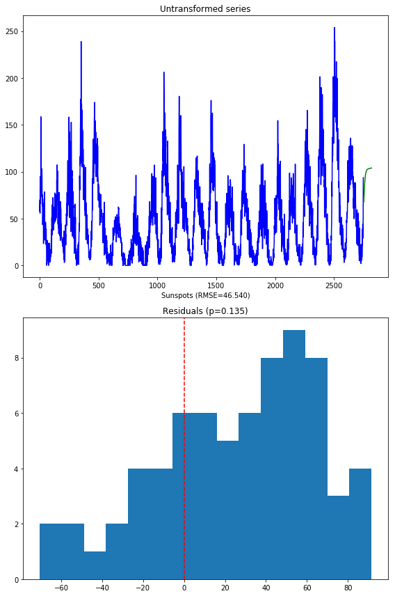
Notice that we are not using the SMAPE (symmetric mean absolute percentage error) as we normally might, because our time series contains zeros. When the actual or forecasted value is zero, SMAPE is known to produce misleadingly large error terms. Instead, we’re using the RMSE.
The second image shows the distribution of the residuals. The normal test shows that they are not normally distributed (which was kind of expected). Here’s what the model over the transformed series produces:
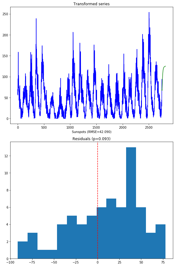
A few things to note:
- These forecasts are on the same scale as the original data. This is because the pipeline is smart enough to inverse transform the forecasts back to the original scale when a transformer is used.
- There is a lower RMSE in the forecasts (also expected, given our hypothesis was that normal data will perform better)
- The residuals are not quite normally distributed, though they are closer than the untransformed model.
8.2.7. Final thoughts
By simply transforming our data prior to fitting our model, we were able to produce
better forecasts (lower RMSE), a more simple model (fewer parameters) that fit significantly
faster, and one that also had a much lower AIC. The key to take away from this is that,
although convenient, the pmdarima.arima.auto_arima() method should not be the first
thing you throw at a time series. Take the time to understand your data, clean it up, and make
necessary transformations before you begin training models.