6. Tips to using auto_arima
The auto_arima function fits the best ARIMA model to a univariate time
series according to a provided information criterion (either
AIC,
AICc,
BIC or
HQIC).
The function performs a search (either stepwise or parallelized)
over possible model & seasonal orders within the constraints provided, and selects
the parameters that minimize the given metric.
The auto_arima function can be daunting. There are a lot of parameters to
tune, and the outcome is heavily dependent on a number of them. In this section,
we lay out several considerations you’ll want to make when you fit your ARIMA
models.
6.1. Understand p, d, and q
ARIMA models are made up of three different terms:
- \(p\): The order of the auto-regressive (AR) model (i.e., the number of lag observations). A time series is considered AR when previous values in the time series are very predictive of later values. An AR process will show a very gradual decrease in the ACF plot.
- \(d\): The degree of differencing.
- \(q\): The order of the moving average (MA) model. This is essentially the size of the “window” function over your time series data. An MA process is a linear combination of past errors.
Often times, ARIMA models are written in the form \(ARIMA(p, d, q)\), where a model with no differencing term, e.g., \(ARIMA(1, 0, 12)\), would be an ARMA (made up of an auto-regressive term and a moving average term, but no integrative term, hence no “I”).
In pmdarima.ARIMA, these parameters are specified in the order argument
as a tuple:
order = (1, 0, 12)  # p=1, d=0, q=12
order = (1, 1, 3)  # p=1, d=1, q=3
# etc.
The parameters p and q can be iteratively searched-for with the auto_arima
function, but the differencing term, d, requires a special set of tests of stationarity
to estimate.
6.1.1. Understanding differencing (d)
An integrative term, d, is typically only used in the case of non-stationary
data. Stationarity in a time series indicates that a series’ statistical attributes,
such as mean, variance, etc., are constant over time (i.e., it exhibits low
heteroskedasticity).
A stationary time series is far more easy to learn and forecast from. With the
d parameter, you can force the ARIMA model to adjust for non-stationarity on
its own, without having to worry about doing so manually.
The value of d determines the number of periods to lag the response prior
to computing differences. E.g.,
from pmdarima.utils import c, diff

# lag 1, diff 1
x = c(10, 4, 2, 9, 34)
diff(x, lag=1, differences=1)
# Returns: array([ -6.,  -2.,   7.,  25.], dtype=float32)
Note that lag and differences are not the same!
diff(x, lag=1, differences=2)
# Returns: array([ 4.,  9., 18.], dtype=float32)

diff(x, lag=2, differences=1)
# Returns: array([-8.,  5., 32.], dtype=float32)
The lag corresponds to the offset in the time period lag, whereas the
differences parameter is the number of times the differences are computed.
Therefore, e.g., for differences=2, the procedure is essentially computing
the difference twice:
x = c(10, 4, 2, 9, 34)

# 1
x_lag = x[1:]  # first lag
x = x_lag - x[:-1]  # first difference
# x = [ -6.,  -2.,   7.,  25.]

# 2
x_lag = x[1:]  # second lag
x = x_lag - x[:-1]
# x = [ 4.,  9., 18.]
6.1.2. Enforcing stationarity
The pmdarima.arima.stationarity sub-module defines various tests of stationarity for
testing a null hypothesis that an observable univariate time series is stationary around
a deterministic trend (i.e. trend-stationary).
A time series is stationary when its mean, variance and auto-correlation, etc.,
are constant over time. Many time-series methods may perform better when a time-series
is stationary, since forecasting values becomes a far easier task for a
stationary time series. ARIMAs that include differencing (i.e., d > 0)
assume that the data becomes stationary after differencing. This is called
difference-stationary. Auto-correlation plots are an easy way to determine
whether your time series is sufficiently stationary for modeling. If the plot
does not appear relatively stationary, your model will likely need a
differencing term. These can be determined by using an Augmented Dickey-Fuller
test, or various other statistical testing methods. Note that auto_arima
will automatically determine the appropriate differencing term for you by default.
import pmdarima as pm
from pmdarima import datasets

y = datasets.load_lynx()
pm.plot_acf(y)
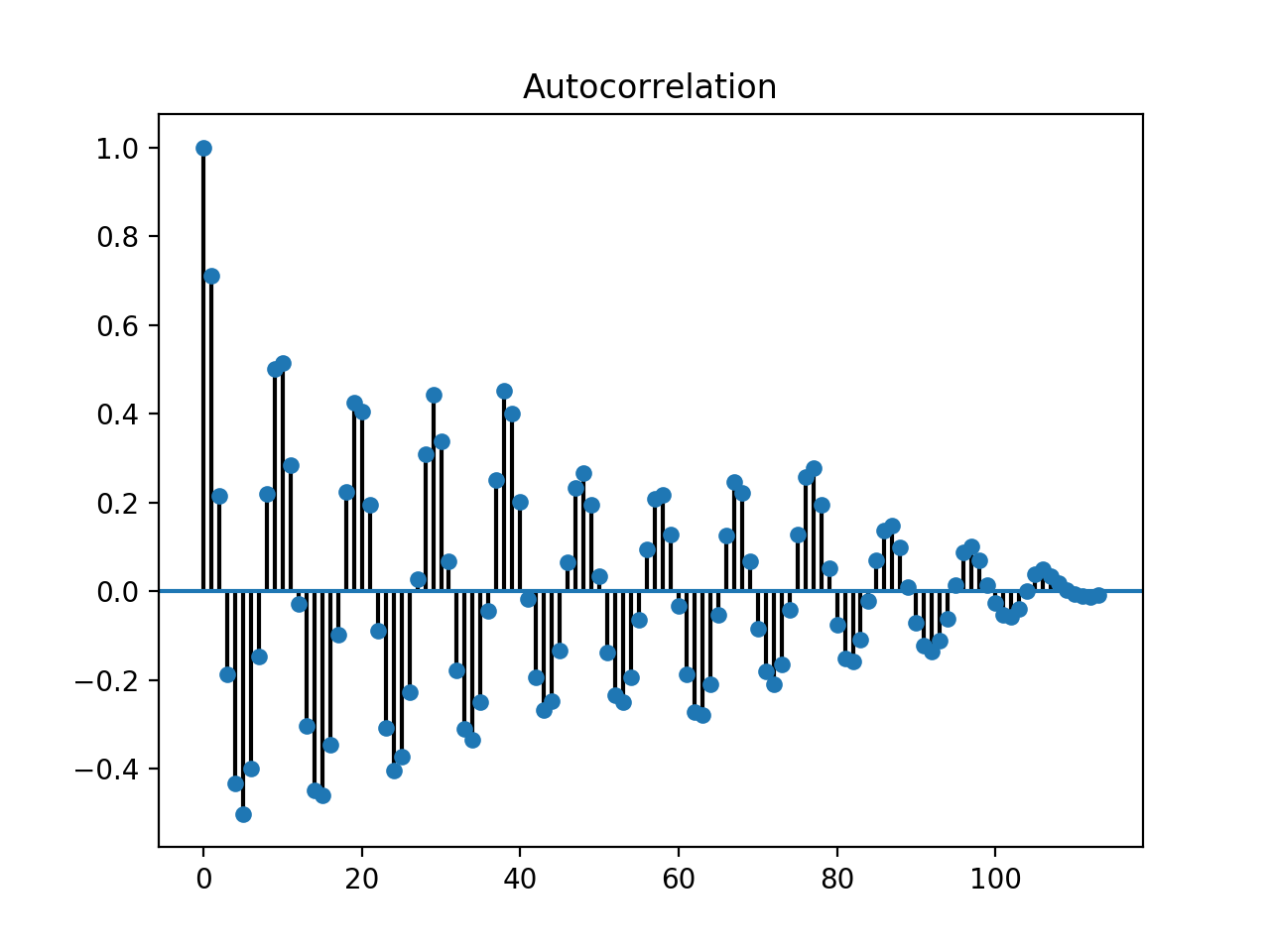
We can examine a time-series’ auto-correlation plot given the code above.
However, to more quantitatively determine whether we need to difference our
data in order to make it stationary, we can conduct a test of stationarity
(either ADFTest, PPTest or KPSSTest).
Each of these tests is based on the R source code, and are primarily intended to be used internally. See this issue for more info. Here’s an example of an ADF test:
from pmdarima.arima.stationarity import ADFTest

# Test whether we should difference at the alpha=0.05
# significance level
adf_test = ADFTest(alpha=0.05)
p_val, should_diff = adf_test.should_diff(y)  # (0.01, False)
The verdict, per the ADF test, is that we should not difference. Pmdarima also
provides a more handy interface for estimating your d parameter more directly.
This is the preferred public method for accessing tests of stationarity:
from pmdarima.arima.utils import ndiffs

# Estimate the number of differences using an ADF test:
n_adf = ndiffs(y, test='adf')  # -> 0

# Or a KPSS test (auto_arima default):
n_kpss = ndiffs(y, test='kpss')  # -> 0

# Or a PP test:
n_pp = ndiffs(y, test='pp')  # -> 0
assert n_adf == n_kpss == n_pp == 0
The easiest way to make your data stationary in the case of ARIMA models is
to allow auto_arima to work its magic, estimate the appropriate d
value, and difference the time series accordingly. However, other
common transformations for enforcing stationarity include (sometimes in
combination with one another):
- Square root or N-th root transformations
- De-trending your time series
- Differencing your time series one or more times
- Log transformations
Note, however, that a transformation on data as a pre-processing stage will
result in forecasts in the transformed space. When in doubt, let the auto_arima
function do the heavy lifting for you. Read more on difference stationarity
in this Duke article.
6.2. Understand P, D, Q and m
Seasonal ARIMA models have three parameters that heavily resemble our p, d and q
parameters:
P: The order of the seasonal component for the auto-regressive (AR) model.D: The integration order of the seasonal process.Q: The order of the seasonal component of the moving average (MA) model.
P and Q and be estimated similarly to p and q via auto_arima, and
D can be estimated via a Canova-Hansen test, however m generally requires subject matter
knowledge of the data.
6.2.1. Estimating the seasonal differencing term, D
Seasonality can manifest itself in timeseries data in unexpected ways. Sometimes trends are partially dependent on the time of year or month. Other times, they may be related to weather patterns. In either case, seasonality is a real consideration that must be made. The pmdarima package provides a test of seasonality for including seasonal terms in your ARIMA models.
We can use a Canova-Hansen test to estimate our seasonal differencing term:
from pmdarima.datasets import load_lynx
from pmdarima.arima.utils import nsdiffs

# load lynx
lynx = load_lynx()

# estimate number of seasonal differences using a Canova-Hansen test
D = nsdiffs(lynx,
            m=10,  # commonly requires knowledge of dataset
            max_D=12,
            test='ch')  # -> 0

# or use the OCSB test (by default)
nsdiffs(lynx,
        m=10,
        max_D=12,
        test='ocsb')  # -> 0
By default, this will be estimated in auto_arima if seasonal=True. Make
sure to pay attention to the m and the max_D parameters.
6.2.2. Setting m
The m parameter relates to the number of observations per seasonal cycle, and is
one that must be known apriori. Typically, m will correspond to some
recurrent periodicity such as:
- 7 - daily
- 12 - monthly
- 52 - weekly
Depending on how it’s set, it can dramatically impact the outcome of an
ARIMA model. For instance, consider the wineind dataset when fit with
m=1 vs. m=12:
import pmdarima as pm

data = pm.datasets.load_wineind()
train, test = data[:150], data[150:]

# Fit two different ARIMAs
m1 = pm.auto_arima(train, error_action='ignore', seasonal=True, m=1)
m12 = pm.auto_arima(train, error_action='ignore', seasonal=True, m=12)
The forecasts these two models will produce are wildly different (code to reproduce):
import matplotlib.pyplot as plt

fig, axes = plt.subplots(1, 2, figsize=(12, 8))
x = np.arange(test.shape[0])

# Plot m=1
axes[0].scatter(x, test, marker='x')
axes[0].plot(x, m1.predict(n_periods=test.shape[0]))
axes[0].set_title('Test samples vs. forecasts (m=1)')

# Plot m=12
axes[1].scatter(x, test, marker='x')
axes[1].plot(x, m12.predict(n_periods=test.shape[0]))
axes[1].set_title('Test samples vs. forecasts (m=12)')

plt.show()
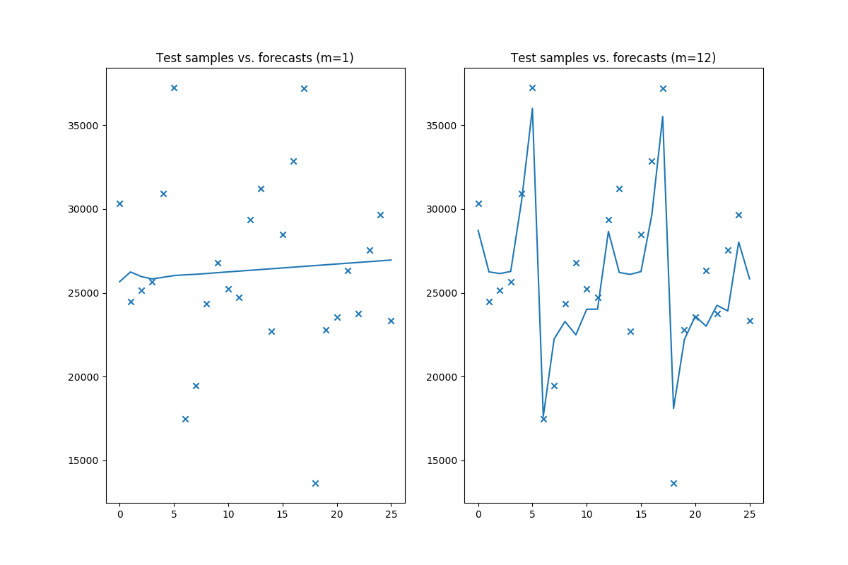
As you can see, depending on the value of m, you may either get a very good model
or a very bad one!!! The author of R’s auto.arima, Rob Hyndman, wrote a very good
blog post on the period
of a seasonal time series.
6.3. Parallel vs. stepwise
The auto_arima function has two modes:
- Stepwise
- Parallelized (slower)
The parallel approach is a naive, brute force grid search over various combinations
of hyper parameters. It will commonly take longer for several reasons. First of all,
there is no intelligent procedure as to how model orders are tested; they are all
tested (no short-circuiting), which can take a while. Second, there is more overhead
in model serialization due to the method in which joblib parallelizes operations.
The stepwise approach follows the strategy laid out by Hyndman and Khandakar in their 2008 paper, “Automatic Time Series Forecasting: The forecast Package for R”.
Step 1: Try four possible models to start:
- \(ARIMA(2, d, 2)\) if
m = 1and \(ARIMA(2, d, 2)(1, D, 1)\) ifm > 1- \(ARIMA(0, d, 0)\) if
m = 1and \(ARIMA(0, d, 0)(0, D, 0)\) ifm > 1- \(ARIMA(1, d, 0)\) if
m = 1and \(ARIMA(1, d, 0)(1, D, 0)\) ifm > 1- \(ARIMA(0, d, 1)\) if
m = 1and \(ARIMA(0, d, 1)(0, D, 1)\) ifm > 1
The model with the smallest AIC (or BIC, or AICc, etc., depending on the minimization criteria) is selected. This is the “current best” model.
Step 2: Consider a number of other models:
- Where one of \(p\), \(q\), \(P\) and \(Q\) is allowed to vary by \(\pm 1\) from the current best model
- Where \(p\) and \(q\) both vary by \(\pm 1\) from the current best model
- Where \(P\) and \(Q\) both vary by \(\pm 1\) from the current best model
Whenever a model with a lower information criteria is found, it becomes the new current best model,
and the procedure is repeated until it cannot find a model close to the current best model
with a lower information criterion or the process exceeds one of the execution thresholds set via arima.StepwiseContext.
When in doubt, stepwise=True is encouraged.
6.3.1. Using StepwiseContext
The StepwiseContext can be used to set the maximum number of steps and/or duration for the stepwise approach.
Please note that these are soft limits that are checked periodically during the stepwise search. The search will be
stopped as soon as one of the thresholds are hit, and the best fit model at that time is returned. This may be helpful
in scenarios that need to balance between best fit model and time constraints.
import pmdarima as pm
from pmdarima.arima import StepwiseContext

data = pm.datasets.load_wineind()
train, test = data[:150], data[150:]

with StepwiseContext(max_dur=15):
    model = pm.auto_arima(train, stepwise=True, error_action='ignore', seasonal=True, m=12)
6.3.2. Other performance concerns
Fitting large models can take some time, and the amount of time tends to scale with m.
If you are fitting a very large set of models, there are some things you can do to
speed things up (at the cost of precision, of course):
- Make sure you have the right value for
m. If you get this wrong, not only will your model suffer, it may take a long time to fit. - Use
stepwise. This is always recommended, but double check if speed is a concern. - Use a sane value for
max_p,max_q,max_Pandmax_Q. You don’t need to search too high; those models will likely be very overfit, anyways. - Try using different optimization methods. For instance,
method='nm'seems to perform more quickly than the default ‘lbfgs’, at the cost of higher amounts of approximation. - Reduce the
maxiterkwarg. The default is 50, but reducing it by 10-20 iterations is often a good trade-off between speed and robustness. - Manipulate the
cov_kwds. If you really want to go down the rabbit hole, you can read about the**fit_kwargsavailable to you in theauto_arimafunction on the statsmodels page - Pre-compute
dorD. You can use thepmdarima.arima.ndiffs()andpmdarima.arima.nsdiffs()methods to compute these ahead of time. - Try using exogenous features instead of a seasonal fit. Sometimes, using fourier exogenous
variables will remove the need for a seasonal model. See
pmdarima.preprocessing.FourierFeaturizerfor more information.
6.4. Pipelining
Sometimes, your data will require several transformations before it’s ready to
be modeled-on. Similar to the scikit-learn Pipeline,
we provide our own modeling pipeline (see pmdarima.pipeline: Pipelining transformers & ARIMAs). This will allow
you to stack an arbitrary number of transformations together before being pushed
into an ARIMA or AutoARIMA estimator:
from pmdarima.pipeline import Pipeline
from pmdarima.preprocessing import BoxCoxEndogTransformer
import pmdarima as pm

wineind = pm.datasets.load_wineind()
train, test = wineind[:150], wineind[150:]

pipeline = Pipeline([
    ("boxcox", BoxCoxEndogTransformer()),
    ("model", pm.AutoARIMA(seasonal=True, suppress_warnings=True))
])

pipeline.fit(train)
pipeline.predict(5)
# array([13.47145799, 13.5052802 , 13.49207821, 13.48365086, 13.48874564])
Note that in this case, what you’d get back are the boxcox-transformed predictions. A more extensive example of pipelines can be found in Examples