Displaying key timeseries statistics

Visualizing characteristics of a time series is a key component to effective forecasting. In this example, we’ll look at a very simple method to examine critical statistics of a time series object.

• 
• 

Out:

Data shape: 2820
Data head:
Jan 1749    58.0
Feb 1749    62.6
Mar 1749    70.0
Apr 1749    55.7
May 1749    85.0
dtype: float64

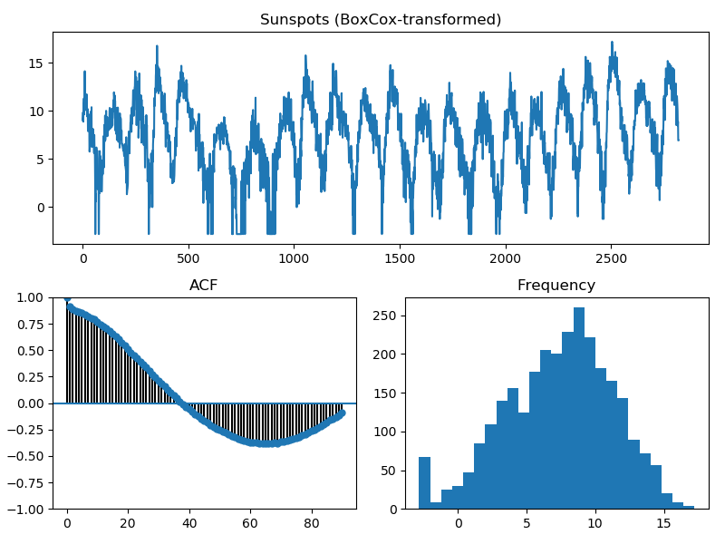
As evidenced by the more normally distributed values in the transformed series,
using a Box-Cox transformation may prove useful prior to fitting your model.

print(__doc__)

# Author: Taylor Smith <taylor.smith@alkaline-ml.com>

import pmdarima as pm
from pmdarima import datasets
from pmdarima import preprocessing

# We'll use the sunspots dataset for this example
y = datasets.load_sunspots(True)
print("Data shape: {}".format(y.shape[0]))
print("Data head:")
print(y.head())

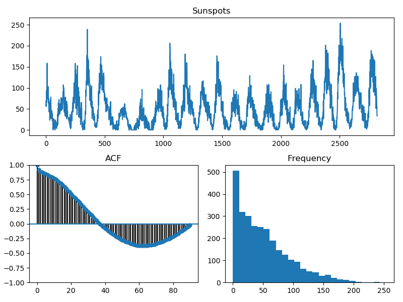
# Let's look at the series, its ACF plot, and a histogram of its values
pm.tsdisplay(y, lag_max=90, title="Sunspots", show=True)

# Notice that the histogram is very skewed. This is a prime candidate for
# box-cox transformation
y_bc, _ = preprocessing.BoxCoxEndogTransformer(lmbda2=1e-6).fit_transform(y)
pm.tsdisplay(
    y_bc, lag_max=90, title="Sunspots (BoxCox-transformed)", show=True)

print("""
As evidenced by the more normally distributed values in the transformed series,
using a Box-Cox transformation may prove useful prior to fitting your model.
""")

Total running time of the script: ( 0 minutes 0.255 seconds)