Pipelines with auto_arima

Like scikit-learn, pmdarima can fit “pipeline” models. That is, a pipeline constitutes a list of arbitrary length comprised of any number of BaseTransformer objects strung together ordinally, and finished with an AutoARIMA object.

The benefit of a pipeline is the ability to condense a complex sequence of stateful transformations into a single object that can call fit, predict and update. It can also be serialized into one pickle file, which greatly simplifies your life.

Out:

pmdarima version: 0.0.0
Performing stepwise search to minimize aic
Fit ARIMA: (2, 1, 2)x(0, 0, 0, 0) (constant=True); AIC=2819.938, BIC=2861.993, Time=0.464 seconds
Fit ARIMA: (0, 1, 0)x(0, 0, 0, 0) (constant=True); AIC=2942.625, BIC=2972.664, Time=0.023 seconds
Fit ARIMA: (1, 1, 0)x(0, 0, 0, 0) (constant=True); AIC=2867.514, BIC=2900.557, Time=0.067 seconds
Fit ARIMA: (0, 1, 1)x(0, 0, 0, 0) (constant=True); AIC=2830.585, BIC=2863.628, Time=0.268 seconds
Fit ARIMA: (0, 1, 0)x(0, 0, 0, 0) (constant=False); AIC=2940.651, BIC=2967.686, Time=0.117 seconds
Fit ARIMA: (1, 1, 2)x(0, 0, 0, 0) (constant=True); AIC=2817.535, BIC=2856.586, Time=0.365 seconds
Fit ARIMA: (0, 1, 2)x(0, 0, 0, 0) (constant=True); AIC=2814.904, BIC=2850.952, Time=0.355 seconds
Fit ARIMA: (0, 1, 3)x(0, 0, 0, 0) (constant=True); AIC=2818.704, BIC=2857.755, Time=0.511 seconds
Fit ARIMA: (1, 1, 1)x(0, 0, 0, 0) (constant=True); AIC=2817.377, BIC=2853.424, Time=0.322 seconds
Fit ARIMA: (1, 1, 3)x(0, 0, 0, 0) (constant=True); AIC=2818.290, BIC=2860.345, Time=0.598 seconds
Near non-invertible roots for order (1, 1, 3)(0, 0, 0, 0); setting score to inf (at least one inverse root too close to the border of the unit circle: 1.000)
Total fit time: 3.095 seconds
Model fit:
Pipeline(steps=[('fourier', FourierFeaturizer(k=4, m=12, prefix=None)),
                ('arima',
                 AutoARIMA(D=None, alpha=0.05, d=None, error_action='ignore',
                           information_criterion='aic', m=1, max_D=1, max_P=2,
                           max_Q=2, max_d=2, max_order=5, max_p=5, max_q=5,
                           maxiter=50, method='lbfgs', n_fits=10, n_jobs=1,
                           offset_test_args=None, out_of_sample_size=0,
                           random=False, random_state=None, scoring='mse',
                           scoring_args=None, seasonal=False,
                           seasonal_test='ocsb', seasonal_test_args=None,
                           start_P=1, start_Q=1, start_p=2, start_params=None, ...))])

Forecasts:
[28518.77767228 29963.38441559 25827.05456596 25060.78046603
 34235.8019525  33509.06300578 21083.18267848 19764.88570594
 25895.79468881 25434.06369412]
[26536.08275776 34421.901483   33695.15536964 21269.27342727
 19950.98131732 26081.88981551 25620.15609753 24414.25585264
 26098.85088839 28871.61206751 30770.63509211]

print(__doc__)

# Author: Taylor Smith <taylor.smith@alkaline-ml.com>

import numpy as np
import pmdarima as pm
from pmdarima import pipeline
from pmdarima import model_selection
from pmdarima import preprocessing as ppc
from pmdarima import arima
from matplotlib import pyplot as plt

print("pmdarima version: %s" % pm.__version__)

# Load the data and split it into separate pieces
data = pm.datasets.load_wineind()
train, test = model_selection.train_test_split(data, train_size=150)

# Let's create a pipeline with multiple stages... the Wineind dataset is
# seasonal, so we'll include a FourierFeaturizer so we can fit it without
# seasonality
pipe = pipeline.Pipeline([
    ("fourier", ppc.FourierFeaturizer(m=12, k=4)),
    ("arima", arima.AutoARIMA(stepwise=True, trace=1, error_action="ignore",
                              seasonal=False,  # because we use Fourier
                              suppress_warnings=True))
])

pipe.fit(train)
print("Model fit:")
print(pipe)

# We can compute predictions the same way we would on a normal ARIMA object:
preds, conf_int = pipe.predict(n_periods=10, return_conf_int=True)
print("\nForecasts:")
print(preds)

# Let's take a look at the actual vs. the predicted values:
fig, axes = plt.subplots(3, 1, figsize=(12, 8))
fig.tight_layout()

# Visualize goodness of fit
in_sample_preds, in_sample_confint = \
    pipe.predict_in_sample(exogenous=None, return_conf_int=True)

n_train = train.shape[0]

x0 = np.arange(n_train)
axes[0].plot(x0, train, alpha=0.75)
axes[0].scatter(x0, in_sample_preds, alpha=0.4, marker='x')
axes[0].fill_between(x0, in_sample_confint[:, 0], in_sample_confint[:, 1],
                     alpha=0.1, color='b')
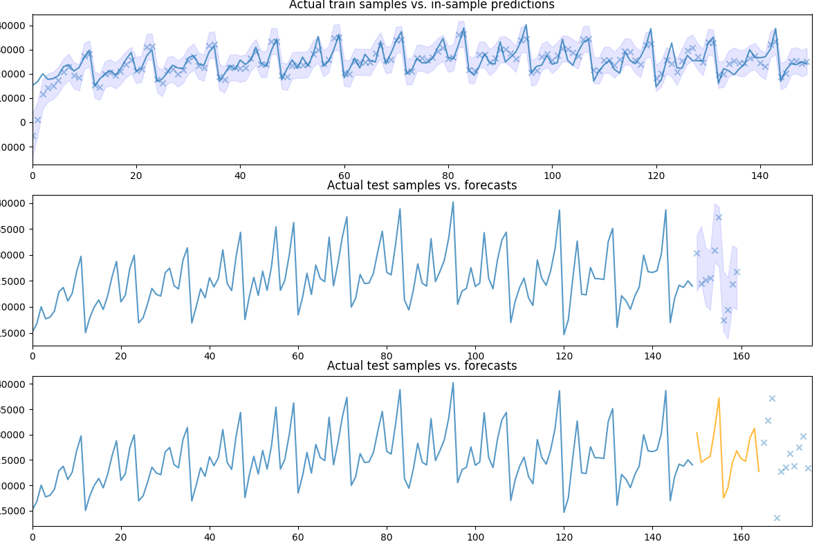
axes[0].set_title('Actual train samples vs. in-sample predictions')
axes[0].set_xlim((0, x0.shape[0]))

# Visualize actual + predicted
x1 = np.arange(n_train + preds.shape[0])
axes[1].plot(x1[:n_train], train, alpha=0.75)
# axes[1].scatter(x[n_train:], preds, alpha=0.4, marker='o')
axes[1].scatter(x1[n_train:], test[:preds.shape[0]], alpha=0.4, marker='x')
axes[1].fill_between(x1[n_train:], conf_int[:, 0], conf_int[:, 1],
                     alpha=0.1, color='b')
axes[1].set_title('Actual test samples vs. forecasts')
axes[1].set_xlim((0, data.shape[0]))

# We can also call `update` directly on the pipeline object, which will update
# the intermittent transformers, where necessary:
newly_observed, still_test = test[:15], test[15:]
pipe.update(newly_observed, maxiter=10)

# Calling predict will now predict from newly observed values
new_preds = pipe.predict(still_test.shape[0])
print(new_preds)

x2 = np.arange(data.shape[0])
n_trained_on = n_train + newly_observed.shape[0]

axes[2].plot(x2[:n_train], train, alpha=0.75)
axes[2].plot(x2[n_train: n_trained_on], newly_observed, alpha=0.75, c='orange')
# axes[2].scatter(x2[n_trained_on:], new_preds, alpha=0.4, marker='o')
axes[2].scatter(x2[n_trained_on:], still_test, alpha=0.4, marker='x')
axes[2].set_title('Actual test samples vs. forecasts')
axes[2].set_xlim((0, data.shape[0]))

plt.show()

Total running time of the script: ( 0 minutes 3.279 seconds)