6. Tips to using `auto_arima`¶

The auto_arima function fits the best ARIMA model to a univariate time series according to either AIC, AICc, BIC or HQIC. The function performs a search (either stepwise or parallelized) over possible model orders within the constraints provided.

The auto_arima function can be daunting. There are a lot of parameters to tune, and the outcome is heavily dependent on a number of them. In this section, we lay out several considerations you’ll want to make when you fit your ARIMA models.

6.1. Understand `p`, `d`, and `q`¶

ARIMA models are made up of three different terms:

p: The order of the auto-regressive (AR) model.
d: The degree of differencing.
q: The order of the moving average (MA) model.

Often times, ARIMA models are written in the form \(ARIMA(p, d, q)\), where a model with no differencing term, e.g., \(ARIMA(1, 0, 12)\), would be an ARMA (made up of an auto-regressive term and a moving average term, but no integrative term).

6.1.1. Understanding differencing¶

An integrative term, d, is typically only used in the case of non-stationary data. The value of d determines the number of periods to lag the response prior to computing differences. E.g.,

from pyramid.utils import c, diff

# lag 1, diff 1
x = c(10, 4, 2, 9, 34)
diff(x, lag=1, differences=1)
# Returns: array([ -6.,  -2.,   7.,  25.], dtype=float32)

Note that lag and differences are not the same!

diff(x, lag=1, differences=2)
# Returns: array([ 4.,  9., 18.], dtype=float32)

diff(x, lag=2, differences=1)
# Returns: array([-8.,  5., 32.], dtype=float32)

The lag corresponds to the offset in the time period lag, whereas the differences parameter is the number of times the differences are computed. Therefore, e.g., for differences=2, the procedure is essentially computing the difference twice:

x = c(10, 4, 2, 9, 34)

# 1
x_lag = x[1:]  # first lag
x = x_lag - x[:-1]  # first difference
# x = [ -6.,  -2.,   7.,  25.]

# 2
x_lag = x[1:]  # second lag
x = x_lag - x[:-1]
# x = [ 4.,  9., 18.]

6.2. Enforcing stationarity¶

The pyramid.arima.stationarity sub-module defines various tests of stationarity for testing a null hypothesis that an observable univariate time series is stationary around a deterministic trend (i.e. trend-stationary).

A time series is stationary when its mean, variance and auto-correlation, etc., are constant over time. Many time-series methods may perform better when a time-series is stationary, since forecasting values becomes a far easier task for a stationary time series. ARIMAs that include differencing (i.e., d > 0) assume that the data becomes stationary after differencing. This is called difference-stationary. Auto-correlation plots are an easy way to determine whether your time series is sufficiently stationary for modeling. If the plot does not appear relatively stationary, your model will likely need a differencing term. These can be determined by using an Augmented Dickey-Fuller test, or various other statistical testing methods. Note that auto_arima will automatically determine the appropriate differencing term for you by default.

import pyramid as pm
from pyramid import datasets

y = datasets.load_lynx()
pm.plot_acf(y)

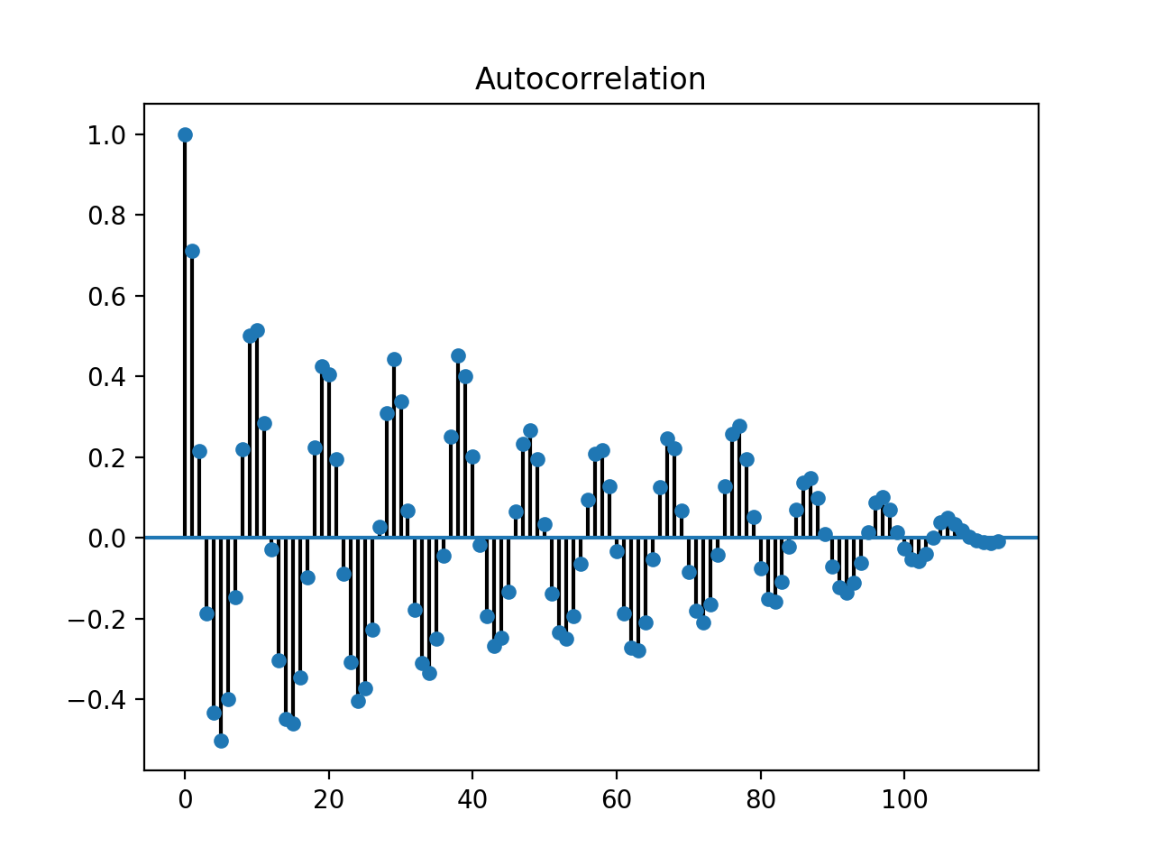
We can examine a time-series’ auto-correlation plot given the code above. However, to more quantitatively determine whether we need to difference our data in order to make it stationary, we can conduct an ADF test:

from pyramid.arima.stationarity import ADFTest

# Test whether we should difference at the alpha=0.05
# significance level
adf_test = ADFTest(alpha=0.05)
p_val, should_diff = adf_test.is_stationary(y)  # (0.99, False)

The verdict, per the ADF test, is that we should not difference. Pyramid also provides a more handy interface for estimating your d parameter more directly:

from pyramid.arima.utils import ndiffs

# Estimate the number of differences using an ADF test:
n_adf = ndiffs(y, test='adf')  # -> 0

# Or a KPSS test (auto_arima default):
n_kpss = ndiffs(y, test='kpss')  # -> 0

# Or a PP test:
n_pp = ndiffs(y, test='pp')  # -> 0
assert n_adf == n_kpss == n_pp == 0

The easiest way to make your data stationary in the case of ARIMA models is to allow auto_arima to work its magic, estimate the appropriate d value, and difference the time series accordingly. However, other common transformations for enforcing stationarity include (sometimes in combination with one another):

Square root or N-th root transformations
De-trending your time series
Differencing your time series one or more times
Log transformations

When in doubt, let the auto_arima function do the heavy lifting for you. Read more on difference stationarity in this Duke article.

6.3. Understand `P`, `D`, `Q` and `m`¶

Seasonal ARIMA models have three parameters that heavily resemble our p, d and q parameters:

P: The order of the seasonal component for the auto-regressive (AR) model.
D: The integration order of the seasonal process.
Q: The order of the seasonal component of the moving average (MA) model.

P and Q and be estimated similarly to p and q via auto_arima, and D can be estimated via a Canova-Hansen test, however m generally requires subject matter knowledge of the data.

6.3.1. Estimating the seasonal differencing term, `D`¶

Seasonality can manifest itself in timeseries data in unexpected ways. Sometimes trends are partially dependent on the time of year or month. Other times, they may be related to weather patterns. In either case, seasonality is a real consideration that must be made. The pyramid package provides a test of seasonality for including seasonal terms in your ARIMA models.

We can use a Canova-Hansen test to estimate our seasonal differencing term:

from pyramid.datasets import load_lynx
from pyramid.arima.utils import nsdiffs

# load lynx
lynx = load_lynx()

# estimate number of seasonal differences
D = nsdiffs(lynx,
            m=10,  # commonly requires knowledge of dataset
            max_D=12,
            test='ch')  # -> 0

By default, this will be estimated in auto_arima if seasonal=True. Make sure to pay attention to the m and the max_D parameters.

6.3.2. Setting `m`¶

The m parameter is the number of observations per seasonal cycle, and is one that must be known apriori. Typically, m will correspond to some recurrent periodicity such as:

7 - daily
12 - monthly
52 - weekly

Depending on how it’s set, it can dramatically impact the outcome of an ARIMA model. For instance, consider the wineind dataset when fit with m=1 vs. m=12:

import pyramid as pm

data = pm.datasets.load_wineind()
train, test = data[:150], data[150:]

# Fit two different ARIMAs
m1 = pm.auto_arima(train, error_action='ignore', seasonal=True, m=1)
m12 = pm.auto_arima(train, error_action='ignore', seasonal=True, m=12)

The forecasts these two models will produce are wildly different (code to reproduce):

import matplotlib.pyplot as plt

fig, axes = plt.subplots(1, 2, figsize=(12, 8))
x = np.arange(test.shape[0])

# Plot m=1
axes[0].scatter(x, test, marker='x')
axes[0].plot(x, m1.predict(n_periods=test.shape[0]))
axes[0].set_title('Test samples vs. forecasts (m=1)')

# Plot m=12
axes[1].scatter(x, test, marker='x')
axes[1].plot(x, m12.predict(n_periods=test.shape[0]))
axes[1].set_title('Test samples vs. forecasts (m=12)')

plt.show()

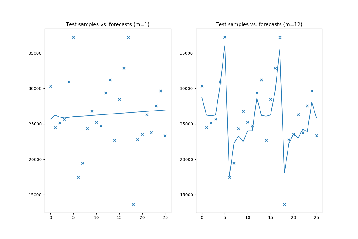
As you can see, depending on the value of m, you may either get a very good model or a very bad one!!! The author of R’s auto.arima, Rob Hyndman, wrote a very good blog post on the period of a seasonal time series.

6.4. Parallel vs. stepwise¶

The auto_arima function has two modes:

Stepwise
Parallelized (slower)

The parallel approach is a naive, brute force grid search over various combinations of hyper parameters. It will commonly take longer for several reasons. First of all, there is no intelligent procedure as to how model orders are tested; they are all tested (no short-circuiting), which can take a while. Second, there is more overhead in model serialization due to the method in which joblib parallelizes operations.

The stepwise approach follows the strategy laid out by Hyndman and Khandakar in their 2008 paper, “Automatic Time Series Forecasting: The forecast Package for R”.

Step 1: Try four possible models to start:

\(ARIMA(2, d, 2)\) if m = 1 and \(ARIMA(2, d, 2)(1, D, 1)\) if m > 1

\(ARIMA(0, d, 0)\) if m = 1 and \(ARIMA(0, d, 0)(0, D, 0)\) if m > 1

\(ARIMA(1, d, 0)\) if m = 1 and \(ARIMA(1, d, 0)(1, D, 0)\) if m > 1

\(ARIMA(0, d, 1)\) if m = 1 and \(ARIMA(0, d, 1)(0, D, 1)\) if m > 1

The model with the smallest AIC (or BIC, or AICc, etc., depending on the minimization criteria) is selected. This is the “current best” model.

Step 2: Consider a number of other models:

Where one of \(p\), \(q\), \(P\) and \(Q\) is allowed to vary by \(\pm 1\) from the current best model

Where \(p\) and \(q\) both vary by \(\pm 1\) from the current best model

Where \(P\) and \(Q\) both vary by \(\pm 1\) from the current best model

Whenever a model with a lower information criteria is found, it becomes the new current best model, and the procedure is repeated until it cannot find a model close to the current best model with a lower information criterion.

When in doubt, stepwise=True is encouraged.

6. Tips to using auto_arima¶

6.1. Understand p, d, and q¶