Modeling quasi-seasonal trends with date features¶

Some trends are common enough to appear seasonal, yet sporadic enough that approaching them from a seasonal perspective may not be valid. An example of this is the “end-of-the-month” effect. In this example, we’ll explore how we can create meaningful features that express seasonal trends without needing to fit a seasonal model.

Out:

pmdarima version: 0.0.0
Head of generated X features:
   DATE-WEEKDAY-0  ...  DATE-DAY-OF-MONTH
0               0  ...                  1
1               0  ...                  2
2               0  ...                  3
3               0  ...                  4
4               0  ...                  5

[5 rows x 8 columns]
Performing stepwise search to minimize aic
Near non-invertible roots for order (2, 1, 2)(0, 0, 0, 0); setting score to inf (at least one inverse root too close to the border of the unit circle: 0.998)
 ARIMA(2,1,2)(0,0,0)[0] intercept   : AIC=inf, Time=3.16 sec
 ARIMA(0,1,0)(0,0,0)[0] intercept   : AIC=2864.731, Time=0.06 sec
First viable model found (2864.731)
 ARIMA(1,1,0)(0,0,0)[0] intercept   : AIC=2861.910, Time=0.75 sec
New best model found (2861.910 < 2864.731)
 ARIMA(0,1,1)(0,0,0)[0] intercept   : AIC=2859.092, Time=1.29 sec
New best model found (2859.092 < 2861.910)
 ARIMA(0,1,0)(0,0,0)[0]             : AIC=2862.772, Time=0.43 sec
Near non-invertible roots for order (1, 1, 1)(0, 0, 0, 0); setting score to inf (at least one inverse root too close to the border of the unit circle: 0.999)
 ARIMA(1,1,1)(0,0,0)[0] intercept   : AIC=inf, Time=1.42 sec
 ARIMA(0,1,2)(0,0,0)[0] intercept   : AIC=2847.648, Time=2.68 sec
New best model found (2847.648 < 2859.092)
Near non-invertible roots for order (1, 1, 2)(0, 0, 0, 0); setting score to inf (at least one inverse root too close to the border of the unit circle: 0.997)
 ARIMA(1,1,2)(0,0,0)[0] intercept   : AIC=inf, Time=2.65 sec
 ARIMA(0,1,3)(0,0,0)[0] intercept   : AIC=2844.490, Time=5.45 sec
New best model found (2844.490 < 2847.648)
Near non-invertible roots for order (1, 1, 3)(0, 0, 0, 0); setting score to inf (at least one inverse root too close to the border of the unit circle: 0.996)
 ARIMA(1,1,3)(0,0,0)[0] intercept   : AIC=inf, Time=5.97 sec
 ARIMA(0,1,4)(0,0,0)[0] intercept   : AIC=2844.554, Time=5.57 sec
 ARIMA(1,1,4)(0,0,0)[0] intercept   : AIC=2846.572, Time=9.24 sec
 ARIMA(0,1,3)(0,0,0)[0]             : AIC=2842.499, Time=3.10 sec
New best model found (2842.499 < 2844.490)
 ARIMA(0,1,2)(0,0,0)[0]             : AIC=2845.649, Time=1.82 sec
 ARIMA(1,1,3)(0,0,0)[0]             : AIC=2840.067, Time=4.27 sec
New best model found (2840.067 < 2842.499)
 ARIMA(1,1,2)(0,0,0)[0]             : AIC=2839.103, Time=1.90 sec
New best model found (2839.103 < 2840.067)
 ARIMA(1,1,1)(0,0,0)[0]             : AIC=2837.109, Time=1.13 sec
New best model found (2837.109 < 2839.103)
 ARIMA(0,1,1)(0,0,0)[0]             : AIC=2857.120, Time=0.77 sec
 ARIMA(1,1,0)(0,0,0)[0]             : AIC=2859.946, Time=0.70 sec
 ARIMA(2,1,1)(0,0,0)[0]             : AIC=2839.104, Time=1.39 sec
 ARIMA(2,1,0)(0,0,0)[0]             : AIC=2854.995, Time=1.26 sec
 ARIMA(2,1,2)(0,0,0)[0]             : AIC=2840.740, Time=2.34 sec

Best model:  ARIMA(1,1,1)(0,0,0)[0]
Total fit time: 57.377 seconds

print(__doc__)

# Author: Taylor Smith <taylor.smith@alkaline-ml.com>

import pmdarima as pm
from pmdarima import arima
from pmdarima import model_selection
from pmdarima import pipeline
from pmdarima import preprocessing
from pmdarima.datasets._base import load_date_example

import numpy as np
from matplotlib import pyplot as plt

print(f"pmdarima version: {pm.__version__}")

# Load the data and split it into separate pieces
y, X = load_date_example()
y_train, y_test, X_train, X_test = \
    model_selection.train_test_split(y, X, test_size=20)

# We can examine traits about the time series:
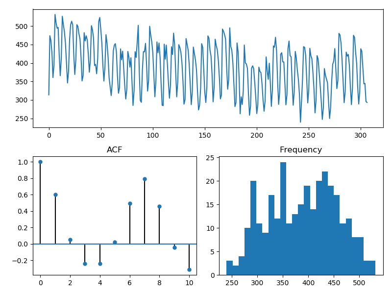
pm.tsdisplay(y_train, lag_max=10)

# We can see the ACF increases and decreases rather rapidly, which means we may
# need some differencing. There also does not appear to be an obvious seasonal
# trend.
n_diffs = arima.ndiffs(y_train, max_d=5)

# Here's what the featurizer will create for us:
date_feat = preprocessing.DateFeaturizer(
    column_name="date",  # the name of the date feature in the X matrix
    with_day_of_week=True,
    with_day_of_month=True)

_, X_train_feats = date_feat.fit_transform(y_train, X_train)
print(f"Head of generated X features:\n{repr(X_train_feats.head())}")

# We can plug this X featurizer into a pipeline:
pipe = pipeline.Pipeline([
    ('date', date_feat),
    ('arima', arima.AutoARIMA(d=n_diffs,
                              trace=3,
                              stepwise=True,
                              suppress_warnings=True,
                              seasonal=False))
])

pipe.fit(y_train, X_train)

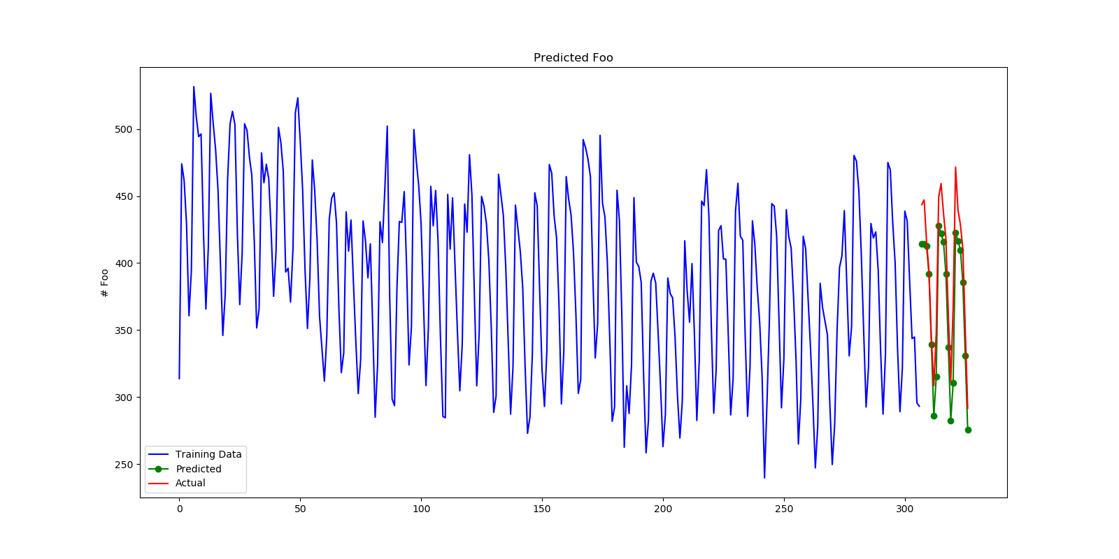
# Plot our forecasts
forecasts = pipe.predict(X=X_test)

fig = plt.figure(figsize=(16, 8))
ax = fig.add_subplot(1, 1, 1)

n_train = y_train.shape[0]
x = np.arange(n_train + forecasts.shape[0])

ax.plot(x[:n_train], y_train, color='blue', label='Training Data')
ax.plot(x[n_train:], forecasts, color='green', marker='o',
        label='Predicted')
ax.plot(x[n_train:], y_test, color='red', label='Actual')
ax.legend(loc='lower left', borderaxespad=0.5)
ax.set_title('Predicted Foo')
ax.set_ylabel('# Foo')

plt.show()

# What next? Try combining different featurizers in your pipeline to enhance
# a model's predictive power.

Total running time of the script: ( 0 minutes 57.821 seconds)

Gallery generated by Sphinx-Gallery