Pipelines with auto_arima

Like scikit-learn, pmdarima can fit “pipeline” models. That is, a pipeline constitutes a list of arbitrary length comprised of any number of BaseTransformer objects strung together ordinally, and finished with an AutoARIMA object.

The benefit of a pipeline is the ability to condense a complex sequence of stateful transformations into a single object that can call fit, predict and update. It can also be serialized into one pickle file, which greatly simplifies your life.

Out:

Fit ARIMA: order=(2, 1, 2); AIC=nan, BIC=nan, Fit time=nan seconds
Fit ARIMA: order=(0, 1, 0); AIC=2942.625, BIC=2972.664, Fit time=0.013 seconds
Fit ARIMA: order=(1, 1, 0); AIC=2844.833, BIC=2877.876, Fit time=0.262 seconds
Fit ARIMA: order=(0, 1, 1); AIC=2809.063, BIC=2842.107, Fit time=0.418 seconds
Fit ARIMA: order=(1, 1, 1); AIC=2783.182, BIC=2819.229, Fit time=0.436 seconds
Fit ARIMA: order=(1, 1, 2); AIC=2812.945, BIC=2851.996, Fit time=0.407 seconds
Fit ARIMA: order=(2, 1, 1); AIC=2784.436, BIC=2823.488, Fit time=0.265 seconds
Total fit time: 1.815 seconds
Model fit:
Pipeline(steps=[('fourier', FourierFeaturizer(k=4, m=12)),
                ('arima',
                 AutoARIMA(D=None, alpha=0.05, callback=None, d=None, disp=0,
                           error_action='ignore', information_criterion='aic',
                           m=1, max_D=1, max_P=2, max_Q=2, max_d=2,
                           max_order=10, max_p=5, max_q=5, maxiter=None,
                           method=None, n_fits=10, n_jobs=1,
                           offset_test_args=None, out_of_sample_size=0,
                           random=False, random_state=None, sarimax_kwargs={},
                           scoring='mse', scoring_args=None, seasonal=False,
                           seasonal_test='ocsb', seasonal_test_args=None,
                           solver='lbfgs', ...))])

Forecasts:
[28520.36805404 29644.13280101 25802.35593918 24894.27891306
 34017.43347142 33378.74778033 21172.88537042 19636.23888839
 25495.03838042 25064.57274529]
[26527.07334287 33561.31009372 33848.84956322 21232.2898864
 19877.75380116 25655.80545853 25261.14297738 24066.66252954
 25770.04805098 28605.9437696  30456.95520294]

print(__doc__)

# Author: Taylor Smith <taylor.smith@alkaline-ml.com>

import numpy as np
import pmdarima as pm
from pmdarima import pipeline, preprocessing as ppc, arima
from matplotlib import pyplot as plt

# Load the data and split it into separate pieces
data = pm.datasets.load_wineind()
train, test = data[:150], data[150:]

# Let's create a pipeline with multiple stages... the Wineind dataset is
# seasonal, so we'll include a FourierFeaturizer so we can fit it without
# seasonality
pipe = pipeline.Pipeline([
    ("fourier", ppc.FourierFeaturizer(m=12, k=4)),
    ("arima", arima.AutoARIMA(stepwise=True, trace=1, error_action="ignore",
                              seasonal=False,  # because we use Fourier
                              transparams=False,
                              suppress_warnings=True))
])

pipe.fit(train)
print("Model fit:")
print(pipe)

# We can compute predictions the same way we would on a normal ARIMA object:
preds, conf_int = pipe.predict(n_periods=10, return_conf_int=True)
print("\nForecasts:")
print(preds)

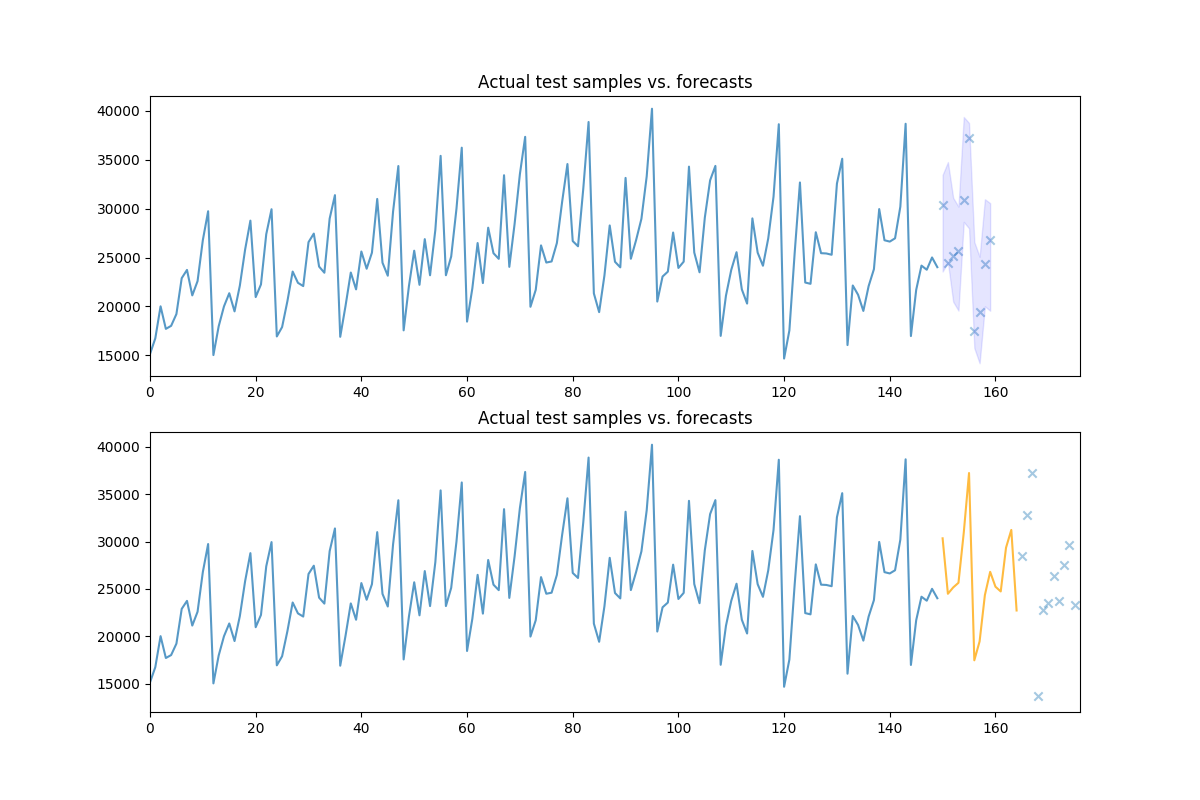
# Let's take a look at the actual vs. the predicted values:
fig, axes = plt.subplots(2, 1, figsize=(12, 8))

n_train = train.shape[0]
x = np.arange(n_train + preds.shape[0])
axes[0].plot(x[:n_train], train, alpha=0.75)
# axes[0].scatter(x[n_train:], preds, alpha=0.4, marker='o')
axes[0].scatter(x[n_train:], test[:preds.shape[0]], alpha=0.4, marker='x')
axes[0].fill_between(x[n_train:], conf_int[:, 0], conf_int[:, 1],
                     alpha=0.1, color='b')
axes[0].set_title('Actual test samples vs. forecasts')
axes[0].set_xlim((0, data.shape[0]))

# We can also call `update` directly on the pipeline object, which will update
# the intermittent transformers, where necessary:
newly_observed, still_test = test[:15], test[15:]
pipe.update(newly_observed, maxiter=10)

# Calling predict will now predict from newly observed values
new_preds = pipe.predict(still_test.shape[0])
print(new_preds)

x2 = np.arange(data.shape[0])
n_trained_on = n_train + newly_observed.shape[0]

axes[1].plot(x2[:n_train], train, alpha=0.75)
axes[1].plot(x2[n_train: n_trained_on], newly_observed, alpha=0.75, c='orange')
# axes[1].scatter(x2[n_trained_on:], new_preds, alpha=0.4, marker='o')
axes[1].scatter(x2[n_trained_on:], still_test, alpha=0.4, marker='x')
axes[1].set_title('Actual test samples vs. forecasts')
axes[1].set_xlim((0, data.shape[0]))

plt.show()

Total running time of the script: ( 0 minutes 1.975 seconds)