Pipelines with auto_arima
Like scikit-learn, pmdarima can fit “pipeline” models. That is, a pipeline
constitutes a list of arbitrary length comprised of any number of
BaseTransformer objects strung together ordinally, and finished with an
AutoARIMA object.
The benefit of a pipeline is the ability to condense a complex sequence of
stateful transformations into a single object that can call fit,
predict and update. It can also be serialized into one pickle file,
which greatly simplifies your life.
Out:
Fit ARIMA: order=(2, 1, 2); AIC=2730.309, BIC=2784.380, Fit time=1.972 seconds
Fit ARIMA: order=(0, 1, 0); AIC=2844.584, BIC=2886.639, Fit time=0.111 seconds
Fit ARIMA: order=(1, 1, 0); AIC=2804.781, BIC=2849.840, Fit time=0.606 seconds
Fit ARIMA: order=(0, 1, 1); AIC=2746.782, BIC=2791.841, Fit time=0.857 seconds
Fit ARIMA: order=(1, 1, 2); AIC=2747.019, BIC=2798.086, Fit time=0.836 seconds
Fit ARIMA: order=(3, 1, 2); AIC=2735.854, BIC=2792.929, Fit time=0.917 seconds
Fit ARIMA: order=(2, 1, 1); AIC=2743.498, BIC=2794.565, Fit time=1.044 seconds
Fit ARIMA: order=(2, 1, 3); AIC=2731.638, BIC=2788.713, Fit time=2.444 seconds
Fit ARIMA: order=(1, 1, 1); AIC=2746.349, BIC=2794.412, Fit time=1.534 seconds
Fit ARIMA: order=(3, 1, 3); AIC=2735.997, BIC=2796.076, Fit time=0.977 seconds
Total fit time: 11.306 seconds
Model fit:
Pipeline(steps=[('fourier', FourierFeaturizer(k=None, m=12)), ('arima', AutoARIMA(D=None, alpha=0.05, callback=None, d=None, disp=0,
     error_action='ignore', information_criterion='aic', m=1, max_D=1,
     max_P=2, max_Q=2, max_d=2, max_order=10, max_p=5, max_q=5,
     maxiter=None, method=None, n_fits=10...ress_warnings=True, test='kpss', trace=1,
     transparams=False, trend=None, with_intercept=True))])

Forecasts:
[28889.17451445 29605.76378588 24962.00313228 26712.98074096
 31501.27998626 36425.54653175 18500.83928146 21530.42884701
 24505.91543048 25208.4774181 ]
[27937.04618389 31376.65591683 36765.81022056 18719.12085696
 21754.59446611 24751.91280803 25435.12411349 24839.30153066
 24712.10330672 29611.43225692 30125.89304143]
print(__doc__)
# Author: Taylor Smith <taylor.smith@alkaline-ml.com>
import numpy as np
import pmdarima as pm
from pmdarima import pipeline, preprocessing as ppc, arima
from matplotlib import pyplot as plt
# Load the data and split it into separate pieces
data = pm.datasets.load_wineind()
train, test = data[:150], data[150:]
# Let's create a pipeline with multiple stages... the Wineind dataset is
# seasonal, so we'll include a FourierFeaturizer so we can fit it without
# seasonality
pipe = pipeline.Pipeline([
("fourier", ppc.FourierFeaturizer(m=12)),
("arima", arima.AutoARIMA(stepwise=True, trace=1, error_action="ignore",
seasonal=False, # because we use Fourier
transparams=False,
suppress_warnings=True))
])
pipe.fit(train)
print("Model fit:")
print(pipe)
# We can compute predictions the same way we would on a normal ARIMA object:
preds, conf_int = pipe.predict(n_periods=10, return_conf_int=True)
print("\nForecasts:")
print(preds)
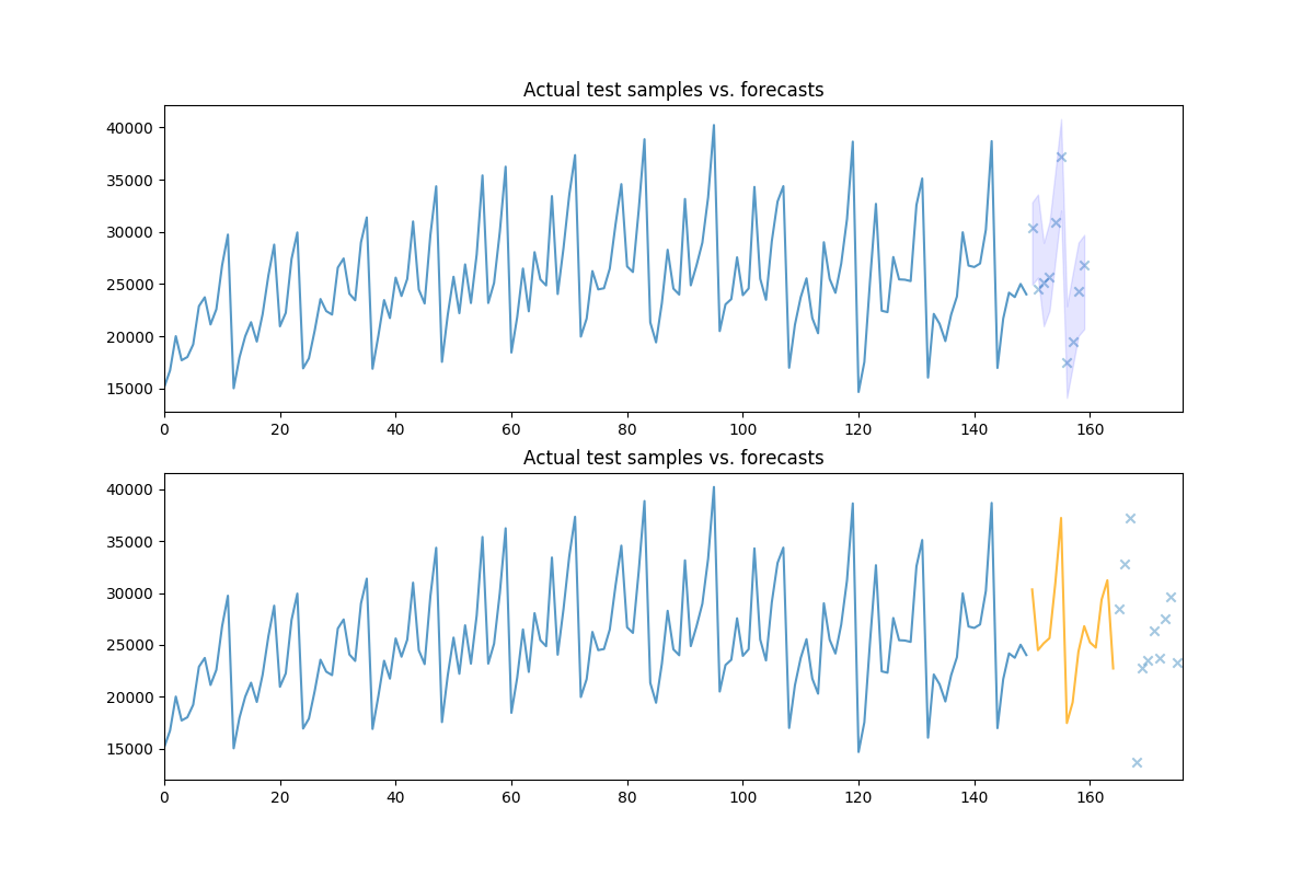
# Let's take a look at the actual vs. the predicted values:
fig, axes = plt.subplots(2, 1, figsize=(12, 8))
n_train = train.shape[0]
x = np.arange(n_train + preds.shape[0])
axes[0].plot(x[:n_train], train, alpha=0.75)
# axes[0].scatter(x[n_train:], preds, alpha=0.4, marker='o')
axes[0].scatter(x[n_train:], test[:preds.shape[0]], alpha=0.4, marker='x')
axes[0].fill_between(x[n_train:], conf_int[:, 0], conf_int[:, 1],
alpha=0.1, color='b')
axes[0].set_title('Actual test samples vs. forecasts')
axes[0].set_xlim((0, data.shape[0]))
# We can also call `update` directly on the pipeline object, which will update
# the intermittent transformers, where necessary:
newly_observed, still_test = test[:15], test[15:]
pipe.update(newly_observed, maxiter=10)
# Calling predict will now predict from newly observed values
new_preds = pipe.predict(still_test.shape[0])
print(new_preds)
x2 = np.arange(data.shape[0])
n_trained_on = n_train + newly_observed.shape[0]
axes[1].plot(x2[:n_train], train, alpha=0.75)
axes[1].plot(x2[n_train: n_trained_on], newly_observed, alpha=0.75, c='orange')
# axes[1].scatter(x2[n_trained_on:], new_preds, alpha=0.4, marker='o')
axes[1].scatter(x2[n_trained_on:], still_test, alpha=0.4, marker='x')
axes[1].set_title('Actual test samples vs. forecasts')
axes[1].set_xlim((0, data.shape[0]))
plt.show()
Total running time of the script: ( 0 minutes 11.993 seconds)